

DNAtlas: Towards Intrinsically Interpretable DNA Language Models
Abstract
DNA language models can determine the pathogenicity of mutations without supervision and generate viable genomes. If the representations learned by DNA language models could be made interpretable, they could augment existing knowledge, provide testable hypotheses or surface previously unknown biology. In this report, we introduce DNAtlas, a minimal convolutional architecture with a novel activation function designed to elicit interpretable neurons, and analyze the representations it learns when pretrained on enterobacterial genomes. We find that simply visualizing the Gram matrix of the activations yields a rich window into the structure of both the DNA being represented and the representation itself. These representations vary substantially across each base in a codon, and their similarities often most visibly depend on relative positional offset, complicating the view of features as directions. Furthermore, we demonstrate the existence of interpretable neurons corresponding to several concepts of interest. Several of our findings are difficult to reconcile with current best practices for interpreting and evaluating DNA language model activations; we offer recommendations accordingly.
Introduction
To rationally engineer biology, one must first understand it. It is understood incompletely, not for lack of effort, and engineered haphazardly. For example, an attempt to remove seven codons from the E. coli genome encountered frequent lethality issues due to unannotated proteins and the introduction of cryptic promoters [1]. The cumulative effects of many small genetic changes can be similarly dramatic for human biology. Genome-wide association studies can find thousands of alleles correlated with disease, but it remains difficult to separate causal alleles from correlated ones or go from causation to mechanistic hypotheses [2, 3].
Since the discovery of neural scaling laws [4], generative models of DNA have dramatically increased in size and capability. The Evo series of models in particular has enabled feats like zero-shot pathogenicity scoring and even generating viable bacteriophage genomes [5, 6, 7]. These models may have acquired a latent understanding of fitness landscapes and the organization of DNA to achieve this. However, how this knowledge is structured in the models is unclear.
Mechanistic interpretability is the science of identifying how deep learning models structure their knowledge. The linear representation hypothesis is a leading explanation for how this is achieved in general [8]. In this framework, neural networks generally learn linear directions in activation space that correspond to interpretable concepts. If only a few features are active at a time, there may be many more features than there are dimensions; this in turn is the superposition hypothesis.
The superposition hypothesis has led to the development of sparse autoencoders (SAEs) [9]. SAEs have underpinned several recent studies interpreting biological foundation models, including InterProt, InterPLM, and Evo 2 itself [10, 11, 6]. These studies have respectively demonstrated that SAE latents can be used to enable interpretable linear regression, fill gaps in existing databases, and create visualizations of bacterial DNA.
Despite these successes, SAEs have recently come under scrutiny. SAE latents often appear to themselves be compositions of a smaller number of interpretable features [12]. Additionally, large language models appear to encode some information in multidimensional structures; these feature manifolds challenge the linear ansatz of SAEs1 [13]. Furthermore, SAEs do not perfectly reconstruct the activations in language models. The remaining "dark matter" is not itself amenable to analysis by SAEs [14]. If this dark matter contains interpretable structure that is simply not compatible with a linear decomposition, SAEs themselves will give no signal of that.
Consistent with prior work across biological sequence modalities, we found that Transformers were outperformed by convolutional models on untokenized DNA, even simple ones [15, 16, 17, 18]. If the inductive biases of Transformers are not optimal for DNA, interpretability methods developed for Transformers and their motivating assumptions may fail to transfer as well.
We believe that it is premature to apply decomposition methods like SAEs to extremely large and heterogeneous DNA models. Some of the strongest early evidence in favor of linear representations came from extensive manual analysis of tiny (by today's standards) convolutional networks, which demonstrated the existence of interpretable neurons2 [19]. The same exercise should be performed with a DNA model.
We ask: do there exist extremely simple architectures that train stably on DNA? Can these models be engineered so that, all else equal, they are easier to interpret? Can we gain substantial insight into the structure of their activations without resorting to either endless per-neuron case studies or decomposition? Can we interpret the DNA itself by observing the activations?
In this work, we answer these questions in the affirmative. Our contributions include:
-
We provide an extremely simple architecture for DNA sequence modeling. We simply replace one branch of a gated MLP with a fully-connected dilated convolution.
-
We engineer the activation function to encourage a greater degree of interpretability.
-
We demonstrate that the Gram matrix of the activations is highly effective at revealing the structure of both the activations themselves and the DNA they represent.
-
This also uncovers some unexpected phenomena: each nucleotide in a codon contains a distinct representation. Furthermore, the similarity between activations is often strongly dependent on their offset, which complicates the view of features as directions.
-
-
We demonstrate the existence of monosemantic neurons corresponding to interesting concepts.
Additionally, we introduce Windowed MLM, a simple objective which enables the model to learn codon-level (and, correspondingly, amino-acid-level) probabilities without tokenization or a prespecified reading frame. An investigation of the modeling performance of DNAtlas on protein tasks is left to future work; the purpose of this paper is interpretability.
A numerical benchmark for interpretability would require an accurate understanding of how the activations are structured. This is the very thing we seek to find. To illustrate: we initially considered using linear probes for rho-independent terminators and alpha helices to assess the model. Instead, we found that the model learns to represent hairpins, be they terminators or REP sites, and to use heterogeneous representations within each codon. Had we tried to optimize the model for these metrics, we would have been severely misled.
Consequently, we do not report certain metrics like recovery of known motifs by neurons and strongly caution against their use. Following a call by leading mechanistic interpretability researchers [20], what we sought was the signal of structure, that is what we found, and that is what we here present.
Reproducibility
With standard methods, DNAtlas trains poorly. If you attempt to replicate this work you will encounter substantial difficulties, and your results will not resemble ours. However, a very stable and robust training recipe does exist, and this recipe was used for the models we present. We believe that the novel capabilities of DNAtlas will be net-positive for biosecurity, but until we are certain that the risks from release are responsibly mitigated, we are withholding the model weights and the training recipe.
If you believe that DNAtlas will be beneficial to your work, we encourage you to contact us directly at [email protected].
Methods
Architecture
Mechanistic interpretability methods for the MLP layers of Transformers are particularly well-developed. These include transcoders and emerging weight-based decomposition techniques [21, 22]. We sought to create a simple architecture that closely resembled an MLP and trained well on DNA.
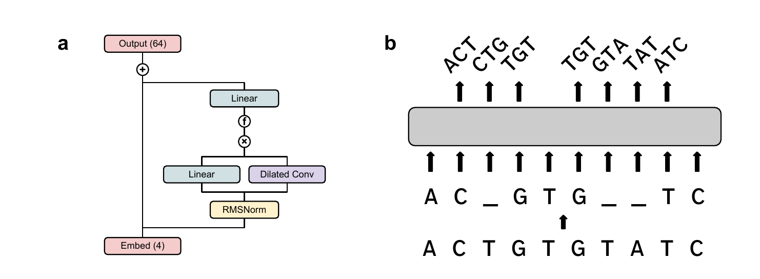
We replaced one branch of a gated MLP with a dense convolution. Dilation is used to extend the context window. Pre-norm is used for stability [23], and an activation function (see Section 3) is added after gating to encourage interpretability. This is the DNAtlas architecture in its entirety (Figure 1).
Hyperparameters are detailed in Appendix B (Table 1). We train two versions of DNAtlas, DNAtlas-Thin and DNAtlas-Wide, which differ in their neuron count: 1024 vs. 3072. All presented interpretability results are for DNAtlas-Wide; forthcoming ablations will be presented for DNAtlas-Thin.
Reverse Complement Equivariance
DNA obeys a global symmetry: every sequence has a reverse complement. Either of the antiparallel strands of the double helix is a valid DNA sequence. If these two views were processed in entirely different ways by the model, this would be problematic for interpretability. Even two qualitatively similar paired features might differ in the way they are computed from the input and the way they affect the output. Learned equivariant families of filters are well known in convolutional models [24], but their empirical existence is not a formal guarantee.
We implemented Reverse Complement Parameter Sharing (RCPS) to resolve this [25]. Convolutional channels are paired up and made mirrors of each other along both the sequence and input channel axes. The same channel-wise pairing and flipping is applied to the embedding and output heads: A with T, ATG with CAT, and so on. From the model's activations on a given input, those on the reverse complement can be derived exactly: swap within each pair and reverse along the sequence axis.
We refer the reader to [26] for a more detailed understanding of how this established technique enables equivariance. Beyond the gains to interpretability, we also found that RCPS improved performance, despite halving the total parameter count (save for a few scalars).
Training
Windowed MLM
We introduce windowed masked language modeling (Figure 1b), a simple modification to ordinary MLM. It appears to train slightly faster than the raw per-nucleotide loss itself and presents no identifiable downsides. We include it in this work due to its performance and to preempt concerns that DNA models cannot be easily compatible with analyses requiring amino-acid-level probabilities. It is not essential for our interpretability results.
While the input is a masked nucleotide sequence, the model predicts the triplet centered at each position. These windows are allowed to overlap. Triplets inconsistent with the input are excluded from consideration by adding a large negative constant to their logits. The loss is computed over every triplet that contains a mask, even if the central nucleotide itself is unmasked.
To compute pseudolikelihoods for all possibilities of a masked codon with per-nucleotide outputs, forward passes are needed: one for each of the 3 positions to be masked and the possible identities of the remaining two. Windowed MLM requires only one forward pass. Amino-acid-wise likelihoods are easily derived at inference time by marginalizing over synonymous codons, once a reading frame is specified. This should enable the straightforward use of techniques like attribution with respect to these likelihoods in future work.
Dataset
We train on the genomes of all type strains in order Enterobacterales (per GTDB [27]) subject to filters, with a sequence length of 4096 and a training/validation split of 95/5. This provides approximately 2.28 billion tokens for training. More details are provided in Appendix C (Table 2).
Activation function
With no nonlinearity, there is little reason to expect the directions of features to be particularly sparse in the neuron basis; we would therefore not expect individual neurons to correspond to particular concepts3. In this section, we describe an activation function which promotes interpretability and the rationale behind it. As previously discussed, it is difficult to construct a numerical benchmark for interpretability without presupposing what features will be learned. Accordingly, this activation was developed through several months of iteration alongside manual investigations into individual neurons. We do not claim uniqueness: many activations may work well. We present one that does.
SoLU
The SoLU+Norm activation was reported by [28] to substantially increase the proportion of neurons with interpretable maximal activations in a language model. This is because as the value of one neuron grows, the values of the remaining neurons are suppressed, encouraging an approximate sparsity. We used this as a starting point to develop an activation that encouraged interpretable neurons.
We swapped LayerNorm for RMSNorm with a single scalar gain [29]. This simply rescales the activations to a fixed magnitude, preserving their direction. In turn, this enables us to easily restrict the activations to be nonnegative.
Nonnegativity
SoLU+Norm with unconstrained inputs frequently produced neurons with interpretable maximum activations. However, it was difficult to relate this interpretation to what was represented by strongly negative activations in general. There did not appear to be a general relationship like antonymy.
To remedy this, we constrained the activations to be nonnegative prior to SoLU. In practice we use (a very weakly) leaky ReLU to prevent the occurrence of dead neurons; this does not seem to otherwise affect the network's behavior. Additionally, we found that nonnegativity was essential to achieving interpretable activation similarity heatmaps. When the similarities are constrained to the range , they can be seen as corresponding to intuitive notions of semantic similarity: from unrelated to identical. Negative similarities, by contrast, lacked a clear general interpretation, besides producing visually jarring heatmaps.
Thresholding
While the SoLU activation prioritizes the most highly active neurons, it would be preferable to have fewer neurons active on any given example to begin with. This suggests the use of a thresholding function. However, we do not want to penalize or restrict large activations per se. A natural choice is then to set every value below a positive threshold to 0, and leave values above it unchanged.
Interestingly, this function has been proposed several times in the literature as an activation function for regularized autoencoders: by [30] as TRec, [31] as ProLU, and [32] as JumpReLU (adapted from [33], who proposed it in the context of adversarial robustness). A symmetric version was proposed by [34] to learn activations with constrained norm.
We use a sigmoid with a learnable strength to approximate the Heaviside function. Together with the leaky ReLU, this yields a function that thresholds strongly below 0 and weakly above it:
Activation similarities
Because the activations are nonnegative and of constant magnitude (we rescale them to unit magnitude without loss of information), their inner product is constrained to . Their Gram matrix, the matrix of pairwise similarities, is readily visualized as an image. We find these to be helpful in determining the structures of both the activations and the DNA itself.
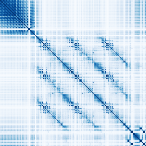

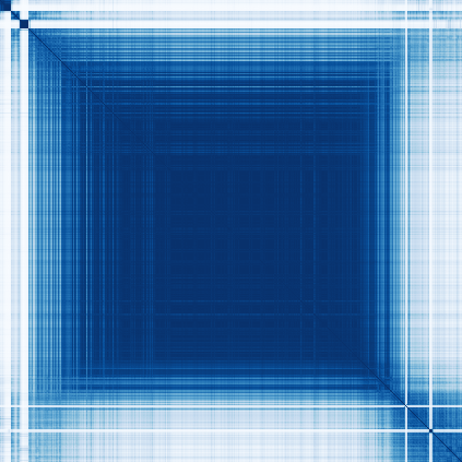

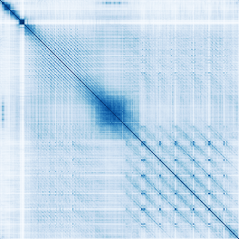
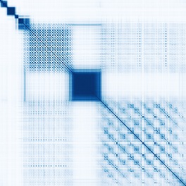
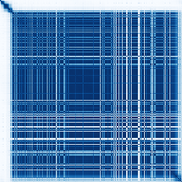
The similarity matrices reveal the organization of the DNA. If directions in activation space correspond to meaningful attributes of DNA, a map of the angular similarities between activations might serve well as a map of those attributes. We find that this is the case: different categories of genomic element appear completely distinct. It is easy to learn to distinguish them at a glance.
Figure 2 presents several examples of this from the E. coli genome. For example, observing panel (a) of Figure 2 from top left to bottom right reveals an oscillating pattern (UP element), two distinctive points (-10 and -35 sites), an intricate pattern repeated three times (each a tRNA), and two pairs of adjacent squares (terminators).
Across every model we have trained, intermediate layers correspond most clearly to abstract concepts. We do not yet have a complete understanding of the early and late layers, though we offer our current impressions in Appendix A and the similarity matrices for every layer in a segment of the Vibrio natriegens genome in Supplementary Figure 1.
The similarity matrices are frequently block-structured. Consider a linear feature activated in two nearby stretches of DNA. We would expect four blocks of similarity: one for each interval with itself and two cross-interval patches. If the activations are collectively well-described by features of this type, be they sparse in the neuron basis or not, their Gram matrix might look like many faint blocks superimposed. This is often seen. For example, CRISPR arrays and REP sites predominantly appear like grids. The csrB noncoding RNA is largely represented by a single direction.
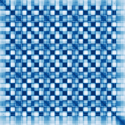
Separate subspaces are learned for the first, second, and third nucleotides in a codon. A close look at any coding region shows a repeating pattern. Every nucleotide is more similar to those a multiple of three away from it than to others. This phenomenon is universal across every version of the model we have trained and across every layer far enough into a model to clearly separate coding from noncoding regions.
The kind of information that each subspace encodes also appears to differ. This is easily visualized by the similarity of every third nucleotide. In this layer, the Gram matrix of the last nucleotide in every codon appears starkly rectangular, suggesting a small number of linear features. Contrastingly, the first and second nucleotides appear to encode similar information, with the first nucleotide's similarities being a "blurry" version of the second's. This is a common arrangement across models we have trained.
Offset-dependent similarity
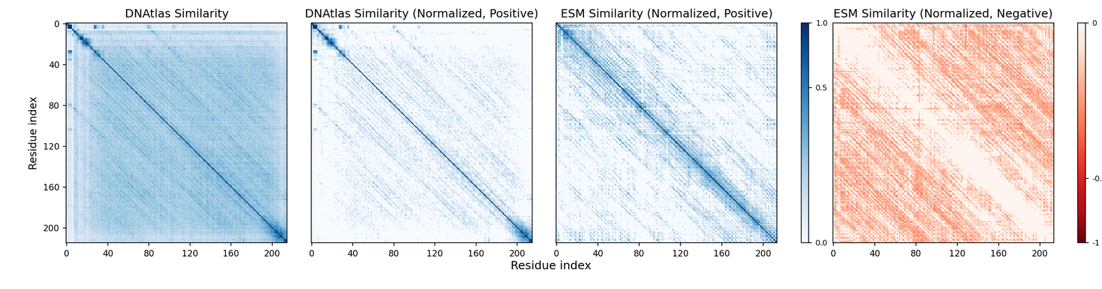
While the similarity matrices are often block-structured, another motif is extremely common across models, layers, and sequences: thin diagonal stripes (resembling a Toeplitz matrix) (Figure 3). These occur particularly commonly in the early layers and in proteins without obvious periodic structure4.
The interpretation follows naturally that the similarity between two nucleotides depends primarily on the distance between them, perhaps conditional upon other attributes. We do not believe that sparsely activated directional features are the canonical explanation for these patterns.
If there are underlying sparse atoms, the activations may be better be modeled as the convolution of them with learned filters. Given that DNAtlas essentially consists of a sparsifying activation function and convolutions, this is not surprising in retrospect. However, it suggests that architectural changes or tailored decomposition methods will be necessary to dissect the activations.
To determine whether this pattern is specific to our setup or might reflect broader tendencies across biological sequence models, we investigated a protein language model: ESM-C-300M. This model differs from ours in architecture, modeling domain, dataset, and training scale. In addition, we inspect the residual as opposed to the outputs of any one layer5. Despite this, we find that the Gram matrix of the residual in early layers is also clearly dominated by offset-dependent similarity. This suggests that this structure of representation emerges from the properties of the domain, not the choice of architecture.
Investigating individual neurons
The existence of offset-dependent similarity suggests that a direction (or the activation of a neuron) may not be the canonical form of a feature in many cases. We no longer believe that the activations of the model can be fully understood by inspecting individual neurons or linear combinations thereof. However, we find that interpretable neurons do exist, and that they correspond to several quantities of interest. We present the neurons after thresholding but before SoLU, which is where we find them to be most interpretable.
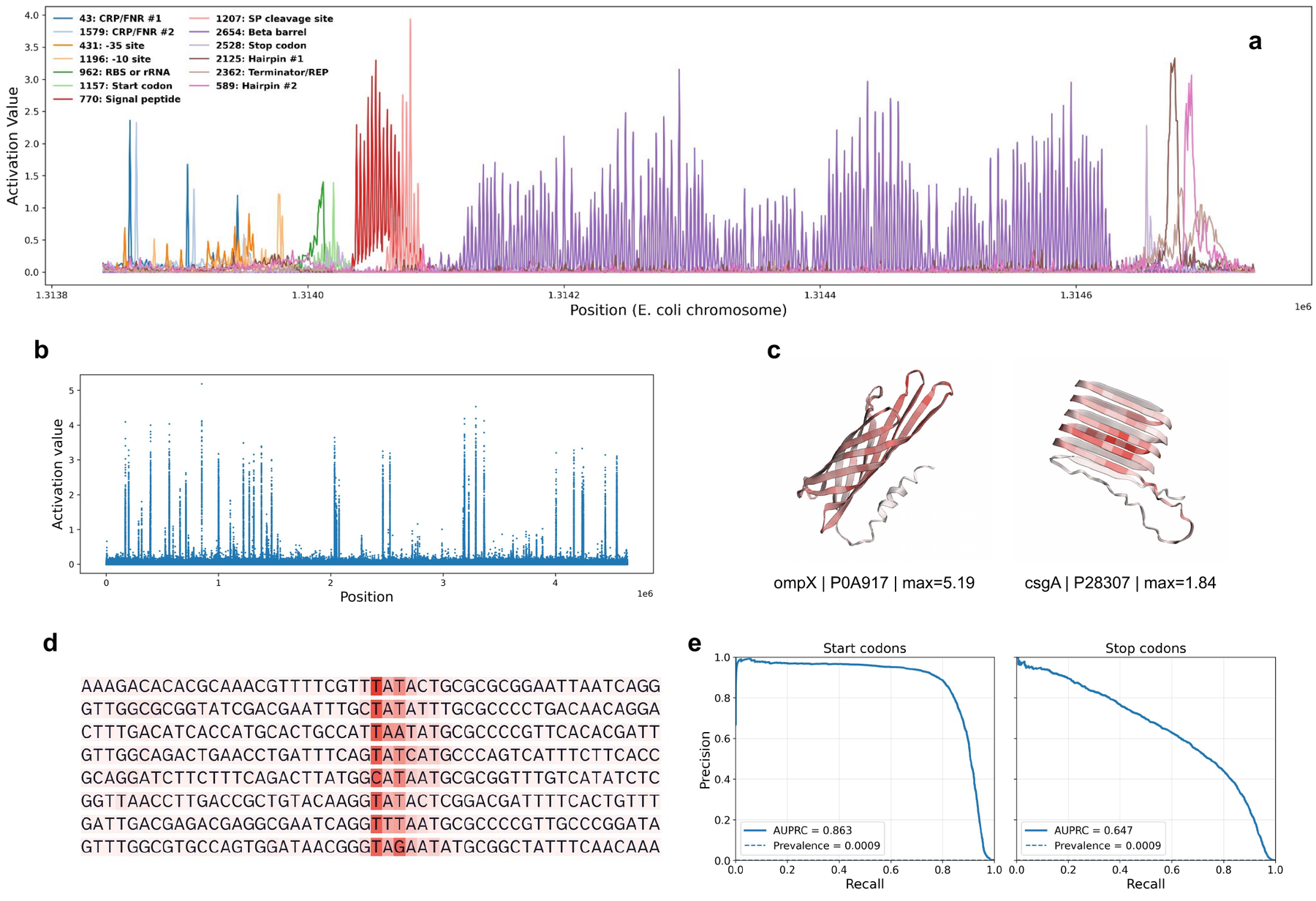
Protein features activate every third nucleotide. The neurons corroborate the heterogeneous representations indicated by the Gram matrices. All investigated protein-related neurons activate with a distinct 3-nucleotide periodicity; counterexamples may exist but we have yet to find any.
Maximal activations are highly distinct. Our activation function was designed to prevent negative activations, suppress weak activations, and leave large activations unchanged. A Manhattan plot easily distinguishes the positions at which neuron 2654 is highly active. The strongest activations are beta barrels, though it also activates more weakly on other structures, like the cross-beta architecture of csgA.
Neurons can be interpreted by analyzing their maximum activations. Neuron 1193, which fires in the region upstream of ompG, clearly corresponds to the -10 site sequence (TATAAT).
Many neurons are interpretable, but their meanings are often surprising. We anticipated finding neurons corresponding to start and stop codons. These do exist6. Neurons 1157 and 2528 achieve an AUPRC of 0.863 and 0.647 with respect to the RefSeq annotations versus 0.0009 expected by chance. However, most of the representations were unexpected. For example, in the visualized window:
-
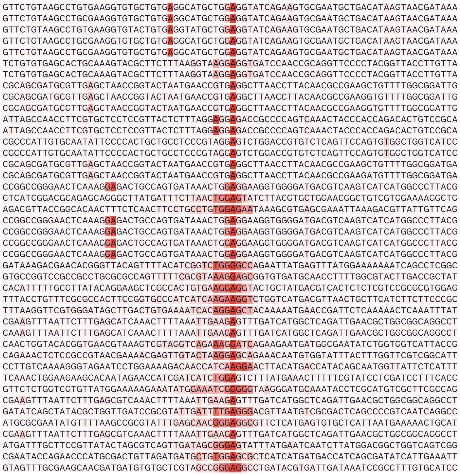
CRP and FNR both recognize 22-base-pair palindromic sites. We find that they are represented by the same two tied pairs of neurons (one pair shown), where each neuron activates on a single nucleotide in the recognition site.
-
A neuron pair is not learned for intrinsic terminators per se but for short palindromes, be they in terminators or REP sites. Another neuron (2326) appears more specific to palindromes that end transcription, many of which are labeled REP sites in EcoCyc [35].
-
Neuron 2525 trails off slowly after each stop codon, though its maximum activations are highly specific for the stop codon itself.
-
While it is easy to describe the maximal activations of neuron 2564, we are unsure what rule excludes beta structures that do not activate it strongly. In turn, we do not know whether this neuron is polysemantic for human-interpretable concepts or monosemantic for an uninterpretable concept.
Monosemantic except for rRNA
We frequently observed throughout development that some otherwise monosemantic neurons activate strongly on rRNA, generally on sequences superficially resembling what they otherwise detect. We provide an example of this in Supplementary Figure 2, where neuron 962 generally detects the Shine-Dalgarno sequence but activates most strongly on 23S rRNA. Ribosomal RNA is long, frequent, and almost perfectly conserved. We currently hypothesize that this phenomenon emerges because it is trivial to get perpetually lower loss on this subset of the broader DNA modeling task.
Ablations
This is a living document. Ablations are forthcoming. In general, we have found that DNAtlas outperforms a strong Transformer baseline (derived by incorporating some techniques from the modded-nanoGPT speedrun) matched roughly for memory and time.
Note that we did not aim for the most efficient architecture per se. We aimed to maximize interpretability while maintaining acceptable performance. There should be straightforward ways to improve the compute efficiency of the model: for example, the addition of attention layers, the use of downsampling, or substituting full for (less expressive) grouped/depthwise convolutions. We chose not to implement these to maintain the homogeneity of the network.
Discussion
With DNAtlas, raw DNA can be converted to interpretable images and per-nucleotide signals with no prior annotations. We believe that offset-dependent similarity implies substantial room for improvement, but these novel capabilities may be of substantial utility to researchers studying difficult-to-cultivate or evolutionarily divergent organisms. Models derived from DNAtlas might be used to visualize mammalian genomes, but this will likely require the incorporation of attention to handle longer contexts.
DNA models are often evaluated on protein-level tasks or for motif prediction by the performance of linear probes applied per-nucleotide. This may not be an appropriate technique if the relevant information is not present at every position. We suggest that using average-pooled activations or a short convolution may be more suitable to evaluate DNA models if their behavior in this respect is not known.
Our work has several limitations. Our understanding of what is learned by the early and late layers in the model is currently much weaker. Additionally, while windowed MLM performs well and has theoretical appeal, we have yet to rigorously evaluate the performance of models trained with it on codon- or protein-level downstream tasks.
We generally found it easy to start with a well-understood sequence, identify highly active neurons, correlate them to known annotations, and establish their monosemanticity or lack thereof. It was often (not always) far more difficult to create a hypothesis for the behavior of a random neuron. This prevented us from calculating metrics such as what proportion of neurons are interpretable. We believe this is possible, but would likely require either substantially improved visualization tools or an agent-based autointerpretation framework. Alternatively, there could be ways to prioritize interesting neurons before interpreting them.
Universality
A close look at Figure 3 reveals not only that offset-dependent similarity is present in both models, but that similar patterns are learned to represent the same protein7. This is despite the substantial differences in architecture, training domain, phylogenetic scope, training scale, loss function, nonnegativity constraint, and location at which the model is investigated. Tentatively, we believe this to be the case in general; we are working to test this result at scale and with more established measures of similarity like CKA [36].
We offer the following hypotheses for future work to operationalize and test:
-
Representations with offset-dependent similarity are not dependent on the architecture, but are, in a sense, Platonic [37]. A property of the biological sequence modeling task necessitates their existence.
-
This property is shift equivariance.
-
Convolutional and state space models can create this representation from the input more readily than Transformers.
-
Standard sparse autoencoders will be of little help to decompose this structure.
-
This structure admits decomposition into interpretable components, but not with standard SAEs.
On the linear representation hypothesis
When all you have are neurons and linear probes, everything interpretable looks like a direction. Investigating what maximizes the activations of single neurons in vision models, as we do in Investigating individual neurons for DNAtlas, was a substantial line of evidence in the development of the linear representation hypothesis [19]. What if we were limited to that analysis?
We would likely have come to the conclusion that some neurons were interpretable, that this linearity could imply the existence of other linear features in superposition, and recommended increasing the width of DNAtlas or considering decomposition. A simple analysis that did not presuppose the geometry of the activations revealed structure that was simple to describe but difficult to reconcile with the features-as-directions view.
We believe that there is substantial utility in investigating directions; the interpretable neurons we have found demonstrate as much. However, as mechanistic interpretability methods are expanded to the sciences, we recommend that similarity-based methods be the primary tools. Methods that presume specific structure in individual activations, including SAEs, should only be used if separate analyses justify the use of the relevant ansatz.
Appendix A — Tacit knowledge
Any machine learning project involves the accumulation of tacit knowledge about the model. This knowledge is often difficult to quantify and present in the context of an academic paper. If it is presented at all, it is usually scattered across companion blog posts, in person talks, and inline comments in code. In this section we share some things we believe are true. Beliefs relating to effective training are omitted for now. We ask that this section be received in the spirit it is presented: a set of informal intuitions and speculations, not ironclad beliefs. Additionally, and in the same informal spirit, we respond to some questions that we might receive.
Things we believe to be true
-
Bidirectional models are not strictly necessary to get a good statistical model of DNA, but the benefits to representation learning are unambiguous. To answer the question what is this nucleotide doing?, there are many cases for which a model of arbitrary genius is less helpful than knowing the next handful of nucleotides, particularly at junctions between segments.
-
MLM/windowed MLM overfits less than autoregressive, probably due to the above.
-
In general, (our impression is that) the functions of the layers are to detect motifs, aggregate motifs into more abstract qualities, model DNA's longer-range colored-noise-like patterns like GC bias [38], and decode the representations into predictions. These functions are not cleanly separated across layers.
-
The high degree of conservation and frequency of rRNA as a portion of the total training data is the cause of many strange issues, but these might yield to a simple solution like logit softcapping.
-
Focal loss for DNA modeling is worth looking into, particularly for autoregressive models, partially as a solution to the above.
-
The general appearance of the activations at a given layer is determined mostly by its position in the stack, less by its dilation.
-
To create a Toeplitz-like Gram matrix while compressing each position to as few neurons as possible, you would have to do something like have a separate neuron for each position that also fires weakly positions ahead of it or behind it. We think this may just be exactly what happens, but are not yet sure.
FAQ
Are the hyperparameters for DNAtlas highly tuned? Many of them are not. For instance, we haven't systematically investigated kernel sizes or learning rate. It doesn't seem particularly sensitive. As we discussed, constructing an interpretability benchmark without (somehow) knowing the structure of the activations in advance is an easy way to fool yourself. This made tuning hyperparameters difficult. Optimizing for performance without considering interpretability would run headlong into Goodhart's Law. However, as a general rule, we kept any change which seemed to improved the performance of the network during development. For example, dilation schedules that repeated more quickly (e.g. 1, 4, 16, 64, 128 vs powers of 2) seemed to learn less "redundant" layers, besides performing better.
How did you decide on the Enterobacterales? They are a well-understood group of simple organisms with many available genomes (orders of magnitude more than what we used to train, though these are concentrated in a few genera and species). It also includes E. coli and V. natriegens, which interest the authors.
Wouldn't an unmasked sequence be highly out of distribution for a model trained on masked sequences? Yes. We tried to account for this with our masking strategy. The parameters of a Markov chain are sampled per-sequence such that of the nucleotides are eligible for masking and the expected run length of ineligible sequence is log-uniform in the range . The probability an eligible nucleotide is actually masked is . This way, the model sees unmasked stretches over many relevant length scales during training. We have yet to compare a model trained in this way to one trained with random masking or any of the many sensible alternatives to this setup.
How was the ompG example chosen? As discussed in the main text, the Gram matrices suggested we might not expect linear features or monosemantic neurons in proteins without periodic structure. During development, we observed that models often dedicate neurons to beta barrels. We thus queried GPT-5 for a simple monocistronic beta barrel in E. coli. Between its suggestions of ompX, ompG, and ompW, we observed that the region around ompG was less cluttered and reasoned it would make a prettier figure. We did not investigate the final training run of DNAtlas to confirm the presence of interpretable neurons in the region before creating the figure, and we didn't have to consider any other proteins to create a presentable figure with what we found.
I think that your results have a clear relationship to group theory/representation theory/sparse coding theory/convolutional sparse coding. Why weren't these discussed in more depth in the paper? The authors do not have the relevant mathematical background to be able to discuss these confidently. We present our empirical results in the hopes that they might be formalized.
Appendix B — Hyperparameters
| Architecture | |
|---|---|
| Model dimension | 512 |
| Layers | 12 |
| Kernel size | 9 |
| Dilation schedule | 1, 4, 16, 64, 128 |
| Expansion factor | 6 |
| Training setup | |
| Sequence length | 4096 |
| Batch size | 96 |
| Total steps | 12000 |
Table 1. Hyperparameters for DNAtlas-Wide. Some hyperparameters relevant for training will remain omitted until we are certain that risks from release are mitigated.
Appendix C — Dataset Criteria
| ALL of | ||
|---|---|---|
| Field | Operator | Value |
| GTDB Taxonomy | contains | Enterobacterales |
| Ambiguous Bases | = | 0 |
| CheckM2 Completeness | > | 98 |
| CheckM2 Contamination | < | 1 |
| GTDB Representative of Species | is | TRUE |
| ANY of | ||
| Assembly Level | is | complete genome |
| Assembly Level | is | chromosome |
Table 2. Criteria used to generate the dataset for training.
Supplementary Figures












A distinction should be made between the views that features are directions and that they exhibit linearity, i.e. that they can be scaled and additively composed. Feature manifolds are not in conflict with linearity, and neither are our results. We generally use the "linear representation hypothesis" to mean the "features as directions hypothesis," in line with common usage. ↩︎
A neuron here refers to a single dimension/channel in the network's activations. These are just particular directions in activation space. ↩︎
In the limit, we would want each feature direction to be unique and 1-sparse, which would yield monosemantic neurons. Below this limit, the behavior may still be useful, for example by learning separate neuron-aligned subspaces for qualitatively distinct information. ↩︎
As opposed to beta-barrels, alpha-helices, et cetera, which do have an obvious periodic structure. ↩︎
We found that we had to mean-center and normalize the activations to obtain a coherent picture, to remove an offset and the effect of a few tokens with very large magnitudes. ↩︎
Albeit with the caveat that the start neuron fires strongly only on the second nucleotide in the codon, and the stop neuron on the first; we use these as targets to calculate AUPRC. ↩︎
As a somewhat ad-hoc measure of similarity, the Spearman correlation between the similarities of the activations in this example, both mean-centered and normalized, excluding the diagonal, is 0.43. ↩︎
References
- A. Nyerges, A. Chiappino-Pepe, B. Budnik, M. Baas-Thomas, R. Flynn, S. Yan, N. Ostrov, M. Liu, M. Wang, Q. Zheng, et al. Synthetic genomes unveil the effects of synonymous recoding. bioRxiv, 2024.
- E. A. Boyle, Y. I. Li, and J. K. Pritchard. An expanded view of complex traits: from polygenic to omnigenic. Cell 169(7):1177–1186, 2017.
- T. Lappalainen, and D. G. MacArthur. From variant to function in human disease genetics. Science 373(6562):1464–1468, 2021.
- J. Kaplan, S. McCandlish, T. Henighan, T. B. Brown, B. Chess, R. Child, S. Gray, A. Radford, J. Wu, and D. Amodei. Scaling Laws for Neural Language Models. arXiv:2001.08361, 2020.
- E. Nguyen, M. Poli, M. G. Durrant, B. Kang, D. Katrekar, D. B. Li, L. J. Bartie, A. W. Thomas, S. H. King, G. Brixi, et al. Sequence modeling and design from molecular to genome scale with Evo. Science 386(6723):eado9336, 2024.
- G. Brixi, M. G. Durrant, J. Ku, M. Poli, G. Brockman, D. Chang, G. A. Gonzalez, S. H. King, D. B. Li, A. T. Merchant, et al. Genome modeling and design across all domains of life with Evo 2. BioRxiv:2025–02, 2025.
- S. H. King, C. L. Driscoll, D. B. Li, D. Guo, A. T. Merchant, G. Brixi, M. E. Wilkinson, and B. L. Hie. Generative design of novel bacteriophages with genome language models. bioRxiv:2025–09, 2025.
- N. Elhage, T. Hume, C. Olsson, N. Schiefer, T. Henighan, S. Kravec, Z. Hatfield-Dodds, R. Lasenby, D. Drain, C. Chen, et al. Toy models of superposition. arXiv preprint arXiv:2209.10652, 2022.
- H. Cunningham, A. Ewart, L. Riggs, R. Huben, and L. Sharkey. Sparse Autoencoders Find Highly Interpretable Features in Language Models. arXiv:2309.08600, 2023.
- E. Adams, L. Bai, M. Lee, Y. Yu, and M. AlQuraishi. From mechanistic interpretability to mechanistic biology: Training, evaluating, and interpreting sparse autoencoders on protein language models. International Conference on Machine Learning (ICML), 2025.
- E. Simon, and J. Zou. Interplm: Discovering interpretable features in protein language models via sparse autoencoders. Nature Methods:1–11, 2025.
- P. Leask, B. Bussmann, M. Pearce, J. Bloom, C. Tigges, N. A. Moubayed, L. Sharkey, and N. Nanda. Sparse Autoencoders Do Not Find Canonical Units of Analysis. arXiv:2502.04878, 2025.
- J. Engels, E. J. Michaud, I. Liao, W. Gurnee, and M. Tegmark. Not All Language Model Features Are One-Dimensionally Linear. arXiv:2405.14860, 2025.
- J. Engels, L. Riggs, and M. Tegmark. Decomposing The Dark Matter of Sparse Autoencoders. arXiv:2410.14670, 2025.
- Y. Bo, W. Mao, Y. Shao, W. Bai, P. Ye, X. Ma, J. Zhao, H. Chen, and C. Shen. Revisiting Convolution Architecture in the Realm of DNA Foundation Models. arXiv:2502.18538, 2025.
- K. K. Yang, N. Fusi, and A. X. Lu. Convolutions are competitive with transformers for protein sequence pretraining. Cell Systems 15(3):286–294, 2024.
- E. Nguyen, M. Poli, M. Faizi, A. Thomas, C. Birch-Sykes, M. Wornow, A. Patel, C. Rabideau, S. Massaroli, Y. Bengio, S. Ermon, S. A. Baccus, and C. Ré. HyenaDNA: Long-Range Genomic Sequence Modeling at Single Nucleotide Resolution. arXiv:2306.15794, 2023.
- Y. Wang, Z. Wang, G. Sadeh, L. Zancato, A. Achille, G. Karypis, and H. Rangwala. LC-PLM: Long-context Protein Language Modeling Using Bidirectional Mamba with Shared Projection Layers. bioRxiv:2024–10, 2024.
- C. Olah, N. Cammarata, L. Schubert, G. Goh, M. Petrov, and S. Carter. Zoom in: An introduction to circuits. Distill 5(3):e00024–001, 2020.
- C. Olah, and A. Jermyn. Reflections on qualitative research. Transformer Circuits Thread, 2024.
- J. Dunefsky, P. Chlenski, and N. Nanda. Transcoders Find Interpretable LLM Feature Circuits. arXiv:2406.11944, 2024.
- L. Bushnaq, D. Braun, and L. Sharkey. Stochastic Parameter Decomposition. arXiv:2506.20790, 2025.
- A. Baevski, and M. Auli. Adaptive input representations for neural language modeling. arXiv preprint arXiv:1809.10853, 2018.
- C. Olah, N. Cammarata, C. Voss, L. Schubert, and G. Goh. Naturally occurring equivariance in neural networks. Distill 5(12):e00024–004, 2020.
- A. Shrikumar, P. Greenside, and A. Kundaje. Reverse-complement parameter sharing improves deep learning models for genomics. bioRxiv, 2017.
- V. Mallet, and J. Vert. Reverse-complement equivariant networks for dna sequences. Advances in neural information processing systems 34:13511–13523, 2021.
- D. H. Parks, M. Chuvochina, C. Rinke, A. J. Mussig, P. Chaumeil, and P. Hugenholtz. GTDB: an ongoing census of bacterial and archaeal diversity through a phylogenetically consistent, rank normalized and complete genome-based taxonomy. Nucleic Acids Research 50(D1):D785–D794, 2022.
- N. Elhage, T. Hume, C. Olsson, N. Nanda, T. Henighan, S. Johnston, S. E. Showk, N. Joseph, N. DasSarma, B. Mann, D. Hernandez, A. Askell, K. Ndousse, A. Jones, D. Drain, A. Chen, Y. Bai, D. Ganguli, L. Lovitt, Z. Hatfield-Dodds, J. Kernion, T. Conerly, S. Kravec, S. Fort, S. Kadavath, J. Jacobson, E. Tran-Johnson, J. Kaplan, J. Clark, T. Brown, S. McCandlish, D. Amodei, and C. Olah. Softmax Linear Units. https://transformer-circuits.pub/2022/solu/index.html, 2022.
- N. Elhage, R. Lasenby, and C. Olah. Privileged bases in the transformer residual stream. Transformer Circuits Thread:24, 2023.
- K. Konda, R. Memisevic, and D. Krueger. Zero-bias autoencoders and the benefits of co-adapting features. International Conference on Learning Representations (ICLR), 2015.
- G. Taggart. ProLU: A Nonlinearity for Sparse Autoencoders. 2024.
- S. Rajamanoharan, T. Lieberum, N. Sonnerat, A. Conmy, V. Varma, J. Kramár, and N. Nanda. Jumping Ahead: Improving Reconstruction Fidelity with JumpReLU Sparse Autoencoders. arXiv:2407.14435, 2024.
- N. B. Erichson, Z. Yao, and M. W. Mahoney. JumpReLU: A Retrofit Defense Strategy for Adversarial Attacks. arXiv:1904.03750, 2019.
- Z. Wang, Q. Ling, and T. S. Huang. Learning Deep $\ell_0$ Encoders. arXiv:1509.00153, 2015.
- L. R. Moore, R. Caspi, D. Boyd, M. Berkmen, A. Mackie, S. Paley, and P. D. Karp. Revisiting the y-ome of Escherichia coli. Nucleic Acids Research 52(20):12201–12207, 2024.
- S. Kornblith, M. Norouzi, H. Lee, and G. Hinton. Similarity of neural network representations revisited. International conference on machine learning:3519–3529, 2019.
- M. Huh, B. Cheung, T. Wang, and P. Isola. The Platonic Representation Hypothesis. arXiv:2405.07987, 2024.
- R. F. Voss. Evolution of long-range fractal correlations and 1/f noise in DNA base sequences. Physical review letters 68(25):3805, 1992.